Hope to have what you need

逻辑回归及python代码实现

    Machine learning     Python·logic regression

  1. 逻辑回归
  2. Sigmoid 函数
  3. 推导过程
    1. 多分类问题
  4. python 实现

逻辑回归

一种广义的线性回归分析模型,逻辑回归虽然带有回归字样,但是逻辑回归属于分类算法。逻辑回归可以进行多分类操作,但由逻辑回归算法本身性质决定其更常用于二分类。

逻辑回归:线性回归可以预测连续值,但是不能解决分类问题,我们需要根据预测的结果判定其属于正类还是负类。所以逻辑回归就是将线性回归的结果,通过 sigmoid 函数映射到 \((0,1)\) 之间。

分类的本质:在空间中找到一个决策边界来完成分类的决策。==逻辑回归的决策边界:可以是非线性的==

Sigmoid 函数

\[g(z)=\frac{1}{1+e^{-z}}\]
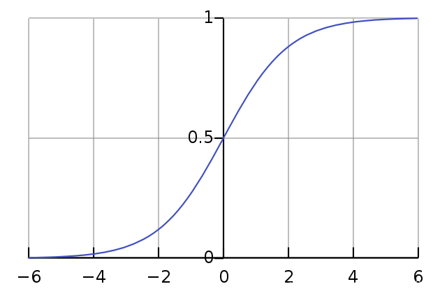
sigmoid

为什么使用 sigmoid 函数

  1. 自变量取值范围任意实数,值域 \([0,1]\),利于分类
  2. 数学特性好,求导容易:\(g′(z)= g(z)\cdot(1-g(z))\)

推导过程

解释:将任意的输入映射到 \([0,1]\) 的区间。我们在线性回归中可以得到一个预测值,再将该值映射到 Sigmoid 函数中,就完成了由值到概率的转换,也就是分类任务

预测函数\(h(\theta)=\frac{1}{1+e^{-\theta^Tx}}\),其中 \(\theta_0+\theta_1x_1+ ... +\theta_nx_n=\displaystyle\sum_{i=1}^n=\theta^Tx\)

分类任务\(\begin{cases} P(y=1|x;\theta)=h_\theta(x) \\ P(y=0|x;\theta)=1-h_\theta(x) \end{cases}\),整合:\(P(y|x;\theta)=(h_\theta(x))^y(1-h_\theta(x))^{1-y}\)

解释:对于二分类任务\((0,1)\),整合后 y 取 0 只保留 \((1-h_\theta(x))^{1-y}\),y 取 1 只保留\((h_\theta(x))^y\)

似然函数\(L(\theta)=\displaystyle\prod_{i=1}^mP(y_i|x_i;\theta)=\displaystyle\prod_{i=1}^m(h_\theta(x_i))^{y_i}(1-h_\theta(x_i))^{1-{y_i}}\)

用对数似然降低复杂度

对数似然\(l(\theta)=\log L(\theta)=\displaystyle\sum_{i=1}^m(y_i\log h_\theta(x_i)+(1-y_i)\log (1-h_\theta(x_i)))\)

此时应用梯度上升求最大值,引入\(J(\theta)=-\frac{1}{m}l(\theta)\),反之梯度下降求最小值

求导过程:

\(\frac{\delta}{\delta_{\theta_j}}J(\theta)=-\frac{1}{m}\displaystyle\sum_{i=1}^m (y_i\frac{1}{h_\theta(x_i)}\frac{\delta}{\delta_{\theta_j}}h_\theta(x_i)-(1-y_i)\frac{1}{1-h_\theta(x_i)}\frac{\delta}{\delta_{\theta_j}}h_\theta(x_i))\)

\(=-\frac{1}{m}\displaystyle\sum_{i=1}^m (y_i\frac{1}{g(\theta^Tx_i)}-(1-y_i)\frac{1}{1-g(\theta^Tx_i)})\frac{\delta}{\delta_{\theta_j}}g(\theta^Tx_i)\)

\(=-\frac{1}{m}\displaystyle\sum_{i=1}^m (y_i\frac{1}{g(\theta^Tx_i)}-(1-y_i)\frac{1}{1-g(\theta^Tx_i)})g(\theta^Tx_i)(1-g(\theta^Tx_i))\frac{\delta}{\delta_{\theta_j}}\theta^Tx_i\)

\(=-\frac{1}{m}\displaystyle\sum_{i=1}^m (y_i(1-g(\theta^Tx_i))-(1-y_i)g(\theta^Tx_i))x_i^j\)

\(=-\frac{1}{m}\displaystyle\sum_{i=1}^m (y_i-g(\theta^Tx_i))x_i^j\)

\(=\frac{1}{m}\displaystyle\sum_{i=1}^m (h_\theta(x_i)-y_i)x_i^j\)

参数更新\(\theta_j:=\theta_j-\alpha\frac{1}{m}\displaystyle\sum_{i=1}^m (h_\theta(x_i)-y_i)x_i^j\)

多分类问题

逻辑回归常用与解决二分类问题,那么它可以用来解决多分类问题吗?

其实也是可以的。之前的逻辑回归可以很好地解决二分类问题,一个样本不是正类就是父类,关于多分类问题的求解可以依靠这个基本原理。常用的多分类思路是“一对多”(one vs all),它的基本思想简单粗暴,构建多个分类器(每个分类器针对一个估计函数)针对每个类别,每个分类器学会识别“是或者不是”该类别,这样就简化为多个二分类问题。用多个逻辑回归作用于待预测样本,返回的最高值作为最后的预测值。

python 实现

通过建立一个逻辑回归模型来预测一个学生是否被大学录取。假设知道两次考试的成绩。有以前的申请人的历史数据,你可以用它作为逻辑回归的训练集,根据考试成绩估计入学概率。

导入所需包

1
2
3
4
import numpy as np
import pandas as pd
import matplotlib.pyplot as plt
import time

读取并查看数据(提取码: v7cd)

1
2
3
4
path = "LogiReg_data.txt"
pdData = pd.read_csv(path, header=None, names=['exam_1', 'exam_2', 'admitted'])
pdData.head()
pdData.shape
    exam_1  exam_2  admitted
0   34.623660   78.024693   0
1   30.286711   43.894998   0
2   35.847409   72.902198   0
3   60.182599   86.308552   1
4   79.032736   75.344376   1
(100, 3)

根据 admitted 画出数据图像

1
2
3
4
5
6
7
8
9
positive = pdData[pdData['admitted'] == 1] # returns the subset of rows such Admitted = 1, i.e. the set of *positive* examples
negative = pdData[pdData['admitted'] == 0] # returns the subset of rows such Admitted = 0, i.e. the set of *negative* examples

plt.subplots(figsize=(10,5))
plt.scatter(positive['exam_1'], positive['exam_2'], s=30, c='b', marker='o', label='Admitted')
plt.scatter(negative['exam_1'], negative['exam_2'], s=30, c='r', marker='x', label='Not Admitted')
plt.legend()
plt.xlabel('Exam_1 Score')
plt.ylabel('Exam_2 Score')
Text(0, 0.5, 'Exam_2 Score')

逻辑回归类

1
2
3
4
5
6
7
8
9
10
11
12
13
14
15
16
17
18
19
20
21
22
23
24
25
26
27
28
29
30
31
32
33
34
35
36
37
38
39
40
41
42
43
44
45
46
47
48
49
50
51
52
53
54
55
56
57
58
59
60
61
62
63
64
65
66
67
68
69
70
71
72
73
74
75
76
77
78
79
80
81
82
83
84
85
86
87
88
89
90
91
92
93
class LogisticRegression():
"""逻辑回归类"""
def __init__(self, n):
self.STOP_ITER = 0
self.STOP_COST = 1
self.STOP_GRAD = 2
self.n = n

def sigmoid(self, z):
"""
sigmoid函数
将预测值映射成概率
"""
return 1 / (1 + np.exp(-z))

def model(self, X, theta):
"""
预测函数:返回预测值
"""
return self.sigmoid(np.dot(X, theta.T))

def cost(self, X, y, theta):
"""损失函数"""
left = np.multiply(-y, np.log(self.model(X, theta)))
right = np.multiply(1 - y, np.log(1 - self.model(X, theta)))
return np.sum(left - right) / (len(X))

def gradient(self, X, y, theta):
"""计算梯度"""
grad = np.zeros(theta.shape)
error = (self.model(X, theta)- y).ravel()
for j in range(len(theta.ravel())): #for each parmeter
term = np.multiply(error, X[:,j])
grad[0, j] = np.sum(term) / len(X)
return grad


def stopCriterion(self, type, value, threshold):
"""
停止标准函数:
1.迭代次数
2.损失值变化
3.梯度变化
"""
if type == self.STOP_ITER:
return value > threshold
elif type == self.STOP_COST:
return abs(value[-1]-value[-2]) < threshold
elif type == self.STOP_GRAD:
return np.linalg.norm(value) < threshold

def shuffleData(self, data):
"""洗牌"""
np.random.shuffle(data)
cols = data.shape[1]
X = data[:, 0:cols-1]
y = data[:, cols-1:]
return X, y

def descent(self, data, theta, batchSize, stopType, thresh, alpha):
"""梯度下降求解"""

init_time = time.time()
i = 0 # 迭代次数
k = 0 # batch
X, y = self.shuffleData(data)
grad = np.zeros(theta.shape) # 计算的梯度
costs = [self.cost(X, y, theta)] # 损失值

while True:
grad = self.gradient(X[k:k+batchSize], y[k:k+batchSize], theta)
k += batchSize #取batch数量个数据
if k >= self.n:
k = 0
X, y = self.shuffleData(data) #重新洗牌
theta = theta - alpha*grad # 参数更新
costs.append(self.cost(X, y, theta)) # 计算新的损失
i += 1

if stopType == self.STOP_ITER:
value = i
elif stopType == self.STOP_COST:
value = costs
elif stopType == self.STOP_GRAD:
value = grad
if self.stopCriterion(stopType, value, thresh):
break

return theta, i-1, costs, grad, time.time() - init_time

def predict(self, X, theta):
return [1 if x >= 0.5 else 0 for x in self.model(X, theta)]

处理数据

1
2
3
4
5
6
7
8
9
10
11
12
13
14
pdData.insert(0, 'Ones', 1) # in a try / except structure so as not to return an error if the block si executed several times

# set X (training data) and y (target variable)
orig_data = pdData.as_matrix() # convert the Pandas representation of the data to an array useful for further computations
cols = orig_data.shape[1]
X = orig_data[:,0:cols-1]
y = orig_data[:,cols-1:cols]

# convert to numpy arrays and initalize the parameter array theta
theta = np.zeros([1, 3])

print(X[:5])
print(y[:5])
print(theta)
array([[ 1.        , 34.62365962, 78.02469282],
       [ 1.        , 30.28671077, 43.89499752],
       [ 1.        , 35.84740877, 72.90219803],
       [ 1.        , 60.18259939, 86.3085521 ],
       [ 1.        , 79.03273605, 75.34437644]])
       array([[0.],
       [0.],
       [0.],
       [1.],
       [1.]])
       array([[0., 0., 0.]])

功能函数

1
2
3
4
5
6
7
8
9
10
11
12
13
14
15
16
17
18
19
20
21
22
23
24
25
26
27
28
29
30
31
lr = LogisticRegression(100)

def runExpe(data, theta, batchSize, stopType, thresh, alpha):

theta, iter, costs, grad, dur = lr.descent(data, theta, batchSize, stopType, thresh, alpha)
print(theta)
name = "Original" if (data[:,1]>2).sum() > 1 else "Scaled"
name += f" data / learning rate: {alpha} / "
if batchSize==1:
strDescType = "Stochastic"
elif batchSize==n:
strDescType = "Gradient"
else:
strDescType = f"Mini-batch ({batchSize})"
name += strDescType + " descent / Stop: "
if stopType == lr.STOP_ITER:
strStop = f"{thresh} iterations"
elif stopType == lr.STOP_COST:
strStop = f"costs change < {thresh}"
else:
strStop = f"gradient norm < {thresh}"
name += strStop
# print(name)
print (f"{name}\nTheta: {theta} / Iter: {iter} / Last cost: {costs[-1]:03.2f} / Duration: {dur:03.2f}s")
plt.subplots(figsize=(12,4))
plt.plot(np.arange(len(costs)), costs, 'r')
plt.xlabel('Iterations')
plt.ylabel('Cost')
plt.xlim(-1,)
plt.title(name.upper())
return theta

基于次数的迭代策略的 batch 梯度下降(5000 次)

1
2
n = 100
theta = runExpe(orig_data, theta, n, 0, thresh=2000, alpha=0.000001)

基于损失值的迭代策略的 batch 梯度下降(109901 次)

1
runExpe(orig_data, theta, n, 1, thresh=0.000001, alpha=0.001)

根据梯度变化停止的 batch 梯度下降(40045 次)

1
runExpe(orig_data, theta, n, 2, thresh=0.05, alpha=0.001)

看一看准确率

1
2
3
4
5
6
7
scaled_X = orig_data[:, :3]
y = orig_data[:, 3]

predictions = lr.predict(scaled_X, theta)
correct = [1 if ((a == 1 and b == 1) or (a == 0 and b == 0)) else 0 for (a, b) in zip(predictions, y)]
accuracy = (sum(map(int, correct)) % len(correct))
print ('accuracy = {0}%'.format(accuracy))
accuracy = 60%

尝试下对数据进行标准化 将数据按其属性(按列进行)减去其均值,然后除以其方差。最后得到的结果是,对每个属性/每列来说所有数据都聚集在 0 附近,方差值为 1

1
2
3
4
from sklearn import preprocessing as pp

scaled_data = orig_data.copy()
scaled_data[:, 1:3] = pp.scale(orig_data[:, 1:3])

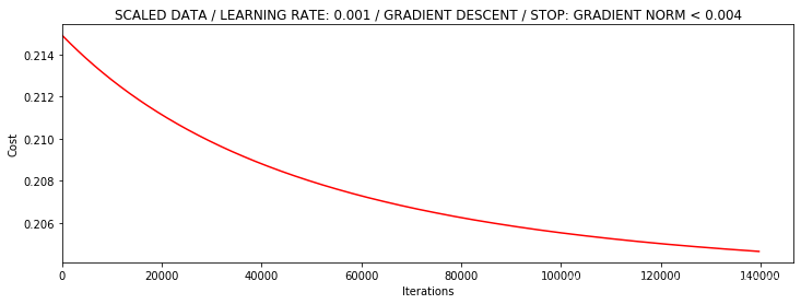
再基于梯度变化停止的 batch 梯度下降(139711 次)

1
runExpe(scaled_data, theta, n, 2, thresh=0.002*2, alpha=0.001)
再基于梯度变化停止的batch梯度下降

基于梯度变化停止的随机梯度下降(72605 次)

1
theta = runExpe(scaled_data, theta, 1, 2, thresh=0.002/5, alpha=0.001)

在看一下准确度

1
2
3
4
5
6
scaled_X = scaled_data[:, :3]
y = scaled_data[:, 3]
predictions = predict(scaled_X, theta)
correct = [1 if ((a == 1 and b == 1) or (a == 0 and b == 0)) else 0 for (a, b) in zip(predictions, y)]
accuracy = (sum(map(int, correct)) % len(correct))
print ('accuracy = {0}%'.format(accuracy))
accuracy = 89%

再基于梯度变化停止的 mini-batch 的梯度下降(3051 次)

1
theta = runExpe(scaled_data, theta, 16, 2, thresh=0.002*2, alpha=0.001)

page PV:  ・  site PV:  ・  site UV: